分析：评估与结果分析

简介

Analysis 模块用于展示日内交易的图形化报告，帮助用户直观地评估和分析投资组合。以下是可查看的图表类型：

• analysis_position

  • report_graph（报告图表）

  • score_ic_graph（IC值图表）

  • cumulative_return_graph（累计收益图表）

  • risk_analysis_graph（风险分析图表）

  • rank_label_graph（排名标签图表）

• analysis_model

  • model_performance_graph（模型性能图表）

Qlib中所有累积收益指标（如收益率、最大回撤）均通过求和方式计算。 这避免了指标或图表随时间呈指数级扭曲。

图形化报告

用户可以运行以下代码获取所有支持的报告：

>> import qlib.contrib.report as qcr
>> print(qcr.GRAPH_NAME_LIST)
['analysis_position.report_graph', 'analysis_position.score_ic_graph', 'analysis_position.cumulative_return_graph', 'analysis_position.risk_analysis_graph', 'analysis_position.rank_label_graph', 'analysis_model.model_performance_graph']

备注

有关更多详细信息，请参考函数文档：类似 help(qcr.analysis_position.report_graph) 的用法

用法与示例

analysis_position.report 的用法

API

qlib.contrib.report.analysis_position.report.report_graph(report_df: DataFrame, show_notebook: bool = True) → [<class 'list'>, <class 'tuple'>]

display backtest report

Example:

import qlib
import pandas as pd
from qlib.utils.time import Freq
from qlib.utils import flatten_dict
from qlib.backtest import backtest, executor
from qlib.contrib.evaluate import risk_analysis
from qlib.contrib.strategy import TopkDropoutStrategy

# init qlib
qlib.init(provider_uri=<qlib data dir>)

CSI300_BENCH = "SH000300"
FREQ = "day"
STRATEGY_CONFIG = {
    "topk": 50,
    "n_drop": 5,
    # pred_score, pd.Series
    "signal": pred_score,
}

EXECUTOR_CONFIG = {
    "time_per_step": "day",
    "generate_portfolio_metrics": True,
}

backtest_config = {
    "start_time": "2017-01-01",
    "end_time": "2020-08-01",
    "account": 100000000,
    "benchmark": CSI300_BENCH,
    "exchange_kwargs": {
        "freq": FREQ,
        "limit_threshold": 0.095,
        "deal_price": "close",
        "open_cost": 0.0005,
        "close_cost": 0.0015,
        "min_cost": 5,
    },
}

# strategy object
strategy_obj = TopkDropoutStrategy(**STRATEGY_CONFIG)
# executor object
executor_obj = executor.SimulatorExecutor(**EXECUTOR_CONFIG)
# backtest
portfolio_metric_dict, indicator_dict = backtest(executor=executor_obj, strategy=strategy_obj, **backtest_config)
analysis_freq = "{0}{1}".format(*Freq.parse(FREQ))
# backtest info
report_normal_df, positions_normal = portfolio_metric_dict.get(analysis_freq)

qcr.analysis_position.report_graph(report_normal_df)

参数:

• report_df --

  df.index.name must be date, df.columns must contain return, turnover, cost, bench.

              return      cost        bench       turnover
  date
  2017-01-04  0.003421    0.000864    0.011693    0.576325
  2017-01-05  0.000508    0.000447    0.000721    0.227882
  2017-01-06  -0.003321   0.000212    -0.004322   0.102765
  2017-01-09  0.006753    0.000212    0.006874    0.105864
  2017-01-10  -0.000416   0.000440    -0.003350   0.208396
  

• show_notebook -- whether to display graphics in notebook, the default is True.

返回:

if show_notebook is True, display in notebook; else return plotly.graph_objs.Figure list.

图形化结果

备注

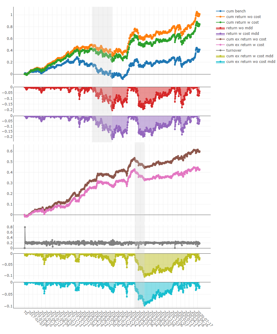
• 横轴 X：交易日

• 纵轴 Y：

  • cum bench

    基准的累计收益序列

  • cum return wo cost

    无成本的投资组合累计收益序列

  • cum return w cost

    有成本的投资组合累计收益序列

  • return wo mdd

    无成本累计收益的最大回撤序列

  • return w cost mdd:

    有成本累计收益的最大回撤序列

  • cum ex return wo cost

    无成本的投资组合相对基准的累计超额收益（CAR）序列

  • cum ex return w cost

    有成本的投资组合相对基准的累计超额收益（CAR）序列

  • turnover

    换手率序列

  • cum ex return wo cost mdd

    无成本累计超额收益（CAR）的回撤序列

  • cum ex return w cost mdd

    有成本累计超额收益（CAR）的回撤序列

• 上方阴影部分：对应 cum return wo cost 的最大回撤

• 下方阴影部分：对应 cum ex return wo cost 的最大回撤

analysis_position.score_ic 的用法

API

qlib.contrib.report.analysis_position.score_ic.score_ic_graph(pred_label: DataFrame, show_notebook: bool = True, **kwargs) → [<class 'list'>, <class 'tuple'>]

分数IC图表

示例:

from qlib.data import D
from qlib.contrib.report import analysis_position
pred_df_dates = pred_df.index.get_level_values(level='datetime')
features_df = D.features(D.instruments('csi500'), ['Ref($close, -2)/Ref($close, -1)-1'], pred_df_dates.min(), pred_df_dates.max())
features_df.columns = ['label']
pred_label = pd.concat([features_df, pred], axis=1, sort=True).reindex(features_df.index)
analysis_position.score_ic_graph(pred_label)

参数:

• pred_label --

  索引为**pd.MultiIndex**，索引名称为**[instrument, datetime]**；列名为**[score, label]**.

  instrument  datetime        score         label
  SH600004  2017-12-11     -0.013502       -0.013502
              2017-12-12   -0.072367       -0.072367
              2017-12-13   -0.068605       -0.068605
              2017-12-14    0.012440        0.012440
              2017-12-15   -0.102778       -0.102778
  

• show_notebook -- whether to display graphics in notebook, the default is True.

返回:

if show_notebook is True, display in notebook; else return plotly.graph_objs.Figure list.

图形化结果

备注

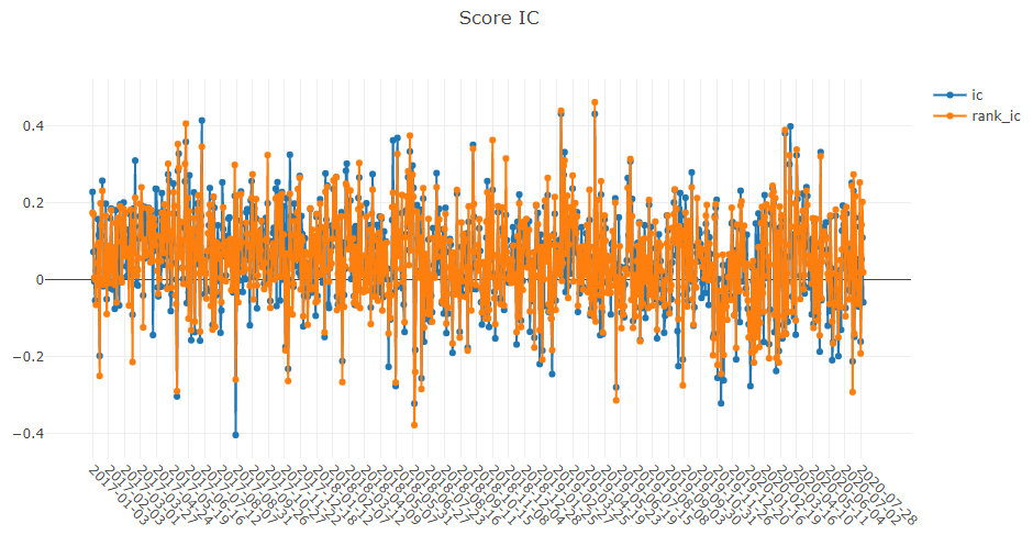
• 横轴 X：交易日

• 纵轴 Y：

  • ic

    label 与 prediction score 之间的皮尔逊相关系数序列。 在上述示例中，label 的计算公式为 Ref($close, -2)/Ref($close, -1)-1。更多详情请参考 数据特征。

  • rank_ic

    label 与 prediction score 之间的斯皮尔曼等级相关系数序列。

analysis_position.risk_analysis 的用法

API

qlib.contrib.report.analysis_position.risk_analysis.risk_analysis_graph(analysis_df: DataFrame = None, report_normal_df: DataFrame = None, report_long_short_df: DataFrame = None, show_notebook: bool = True) → Iterable[Figure]

生成分析图表和月度分析

示例:

import qlib
import pandas as pd
from qlib.utils.time import Freq
from qlib.utils import flatten_dict
from qlib.backtest import backtest, executor
from qlib.contrib.evaluate import risk_analysis
from qlib.contrib.strategy import TopkDropoutStrategy

# 初始化qlib
qlib.init(provider_uri=<qlib数据目录>)

CSI300_BENCH = "SH000300"
FREQ = "day"
STRATEGY_CONFIG = {
    "topk": 50,
    "n_drop": 5,
    # pred_score, pd.Series
    "signal": pred_score,
}

EXECUTOR_CONFIG = {
    "time_per_step": "day",
    "generate_portfolio_metrics": True,
}

backtest_config = {
    "start_time": "2017-01-01",
    "end_time": "2020-08-01",
    "account": 100000000,
    "benchmark": CSI300_BENCH,
    "exchange_kwargs": {
        "freq": FREQ,
        "limit_threshold": 0.095,
        "deal_price": "close",
        "open_cost": 0.0005,
        "close_cost": 0.0015,
        "min_cost": 5,
    },
}

# 策略对象
strategy_obj = TopkDropoutStrategy(**STRATEGY_CONFIG)
# 执行器对象
executor_obj = executor.SimulatorExecutor(** EXECUTOR_CONFIG)
# 回测
portfolio_metric_dict, indicator_dict = backtest(executor=executor_obj, strategy=strategy_obj, **backtest_config)
analysis_freq = "{0}{1}".format(*Freq.parse(FREQ))
# 回测信息
report_normal_df, positions_normal = portfolio_metric_dict.get(analysis_freq)
analysis = dict()
analysis["excess_return_without_cost"] = risk_analysis(
    report_normal_df["return"] - report_normal_df["bench"], freq=analysis_freq
)
analysis["excess_return_with_cost"] = risk_analysis(
    report_normal_df["return"] - report_normal_df["bench"] - report_normal_df["cost"], freq=analysis_freq
)

analysis_df = pd.concat(analysis)  # type: pd.DataFrame
analysis_position.risk_analysis_graph(analysis_df, report_normal_df)

参数:

• analysis_df --

  分析数据，索引为**pd.MultiIndex**；列名为**[risk]**.

                                                    risk
  excess_return_without_cost mean               0.000692
                             std                0.005374
                             annualized_return  0.174495
                             information_ratio  2.045576
                             max_drawdown      -0.079103
  excess_return_with_cost    mean               0.000499
                             std                0.005372
                             annualized_return  0.125625
                             information_ratio  1.473152
                             max_drawdown      -0.088263
  

• report_normal_df --

  df.index.name**必须为**date，df.columns必须包含**return**、turnover、cost、bench.

              return      cost        bench       turnover
  date
  2017-01-04  0.003421    0.000864    0.011693    0.576325
  2017-01-05  0.000508    0.000447    0.000721    0.227882
  2017-01-06  -0.003321   0.000212    -0.004322   0.102765
  2017-01-09  0.006753    0.000212    0.006874    0.105864
  2017-01-10  -0.000416   0.000440    -0.003350   0.208396
  

• report_long_short_df --

  df.index.name**必须为**date，df.columns包含**long**、short、long_short.

              long        short       long_short
  date
  2017-01-04  -0.001360   0.001394    0.000034
  2017-01-05  0.002456    0.000058    0.002514
  2017-01-06  0.000120    0.002739    0.002859
  2017-01-09  0.001436    0.001838    0.003273
  2017-01-10  0.000824    -0.001944   -0.001120
  

• show_notebook -- 是否在notebook中显示图形，默认为**True**. 若为True，在notebook中显示图形 若为False，返回图形对象

返回:

图形对象列表

图形化结果

备注

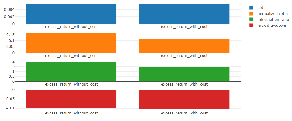
• 通用图表

  • `std`（标准差）

    • excess_return_without_cost

      无成本的累计超额收益（CAR）的标准差。

    • excess_return_with_cost

      有成本的累计超额收益（CAR）的标准差。

  • `annualized_return`（年化收益率）

    • excess_return_without_cost

      无成本的累计超额收益（CAR）的年化收益率。

    • excess_return_with_cost

      有成本的累计超额收益（CAR）的年化收益率。

  • `information_ratio`（信息比率）

    • excess_return_without_cost

      无成本的信息比率。

    • excess_return_with_cost

      有成本的信息比率。

    有关信息比率的更多信息，请参考 信息比率 - IR。

  • `max_drawdown`（最大回撤）

    • excess_return_without_cost

      无成本的累计超额收益（CAR）的最大回撤。

    • excess_return_with_cost

      有成本的累计超额收益（CAR）的最大回撤。

备注

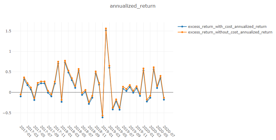
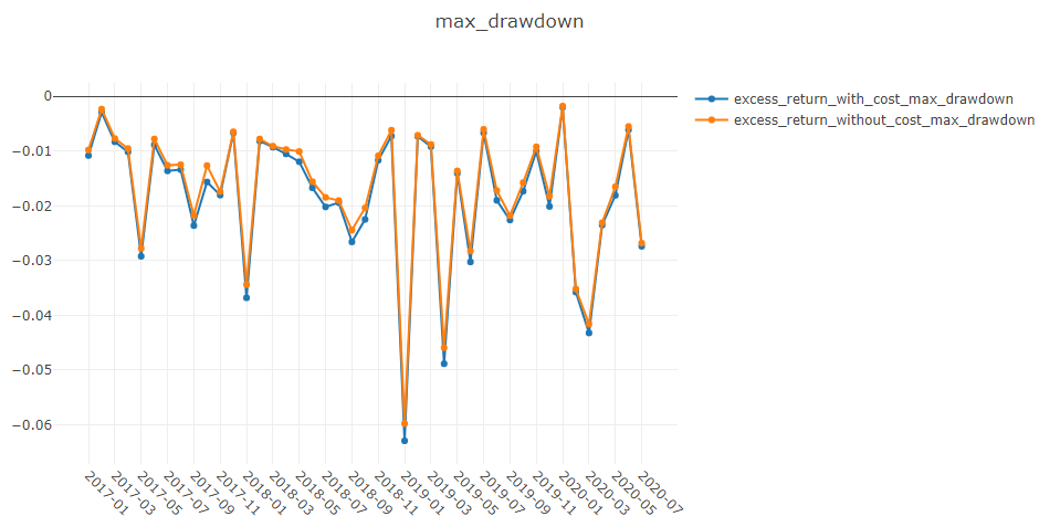
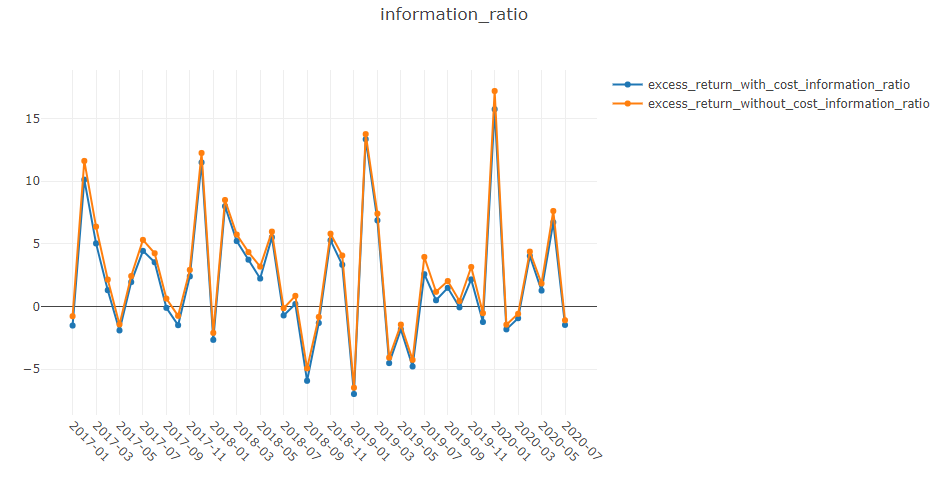
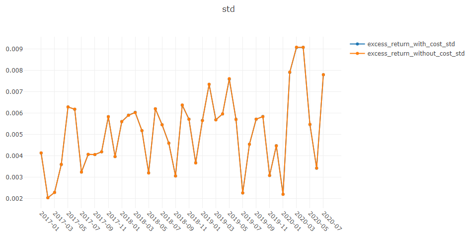
• annualized_return/max_drawdown/information_ratio/std 图表

  • 横轴 X：按月份分组的交易日

  • 纵轴 Y：

    • annualized_return 图表

      • excess_return_without_cost_annualized_return

        无成本的月度累计超额收益（CAR）的年化收益率序列。

      • excess_return_with_cost_annualized_return

        有成本的月度累计超额收益（CAR）的年化收益率序列。

    • max_drawdown 图表

      • excess_return_without_cost_max_drawdown

        无成本的月度累计超额收益（CAR）的最大回撤序列。

      • excess_return_with_cost_max_drawdown

        有成本的月度累计超额收益（CAR）的最大回撤序列。

    • information_ratio 图表

      • excess_return_without_cost_information_ratio

        无成本的月度累计超额收益（CAR）的信息比率序列。

      • excess_return_with_cost_information_ratio

        有成本的月度累计超额收益（CAR）的信息比率序列。

    • std 图表

      • excess_return_without_cost_max_drawdown

        无成本的月度累计超额收益（CAR）的标准差序列。

      • excess_return_with_cost_max_drawdown

        有成本的月度累计超额收益（CAR）的标准差序列。

analysis_model.analysis_model_performance 的用法

API

qlib.contrib.report.analysis_model.analysis_model_performance.ic_figure(ic_df: DataFrame, show_nature_day=True, **kwargs) → Figure

信息系数(IC)图表

参数:

• ic_df -- IC数据框

• show_nature_day -- 是否显示非交易日的横坐标

• **kwargs -- 包含控制Plotly图表样式的参数，目前支持 - rangebreaks: https://plotly.com/python/time-series/#Hiding-Weekends-and-Holidays

返回:

plotly.graph_objs.Figure对象

qlib.contrib.report.analysis_model.analysis_model_performance.model_performance_graph(pred_label: DataFrame, lag: int = 1, N: int = 5, reverse=False, rank=False, graph_names: list = ['group_return', 'pred_ic', 'pred_autocorr'], show_notebook: bool = True, show_nature_day: bool = False, **kwargs) → [<class 'list'>, <class 'tuple'>]

Model performance

参数:

• pred_label --

  index is pd.MultiIndex, index name is [instrument, datetime]; columns names is [score, label]. It is usually same as the label of model training(e.g. "Ref($close, -2)/Ref($close, -1) - 1").

  instrument  datetime        score       label
  SH600004    2017-12-11  -0.013502       -0.013502
                  2017-12-12  -0.072367       -0.072367
                  2017-12-13  -0.068605       -0.068605
                  2017-12-14  0.012440        0.012440
                  2017-12-15  -0.102778       -0.102778
  

• lag -- pred.groupby(level='instrument', group_keys=False)['score'].shift(lag). It will be only used in the auto-correlation computing.

• N -- group number, default 5.

• reverse -- if True, pred['score'] *= -1.

• rank -- if True, calculate rank ic.

• graph_names -- graph names; default ['cumulative_return', 'pred_ic', 'pred_autocorr', 'pred_turnover'].

• show_notebook -- whether to display graphics in notebook, the default is True.

• show_nature_day -- whether to display the abscissa of non-trading day.

• **kwargs -- contains some parameters to control plot style in plotly. Currently, supports - rangebreaks: https://plotly.com/python/time-series/#Hiding-Weekends-and-Holidays

返回:

if show_notebook is True, display in notebook; else return plotly.graph_objs.Figure list.

图形化结果

备注

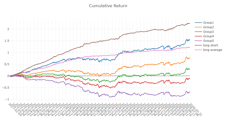
• 累计收益图表

  • Group1:

    `ranking ratio`（标签排名比率）小于等于20%的股票组的累计收益序列

  • Group2:

    20% < `ranking ratio`（标签排名比率）小于等于40%的股票组的累计收益序列

  • Group3:

    40% < `ranking ratio`（标签排名比率）小于等于60%的股票组的累计收益序列

  • Group4:

    60% < `ranking ratio`（标签排名比率）小于等于80%的股票组的累计收益序列

  • Group5:

    `ranking ratio`（标签排名比率）大于80%的股票组的累计收益序列

  • long-short:

    `Group1`与`Group5`累计收益的差值序列

  • long-average

    `Group1`与所有股票累计收益均值的差值序列

  `ranking ratio`（标签排名比率）可表示为：

  \[ranking\ ratio = \frac{Ascending\ Ranking\ of\ label}{Number\ of\ Stocks\ in\ the\ Portfolio}\]

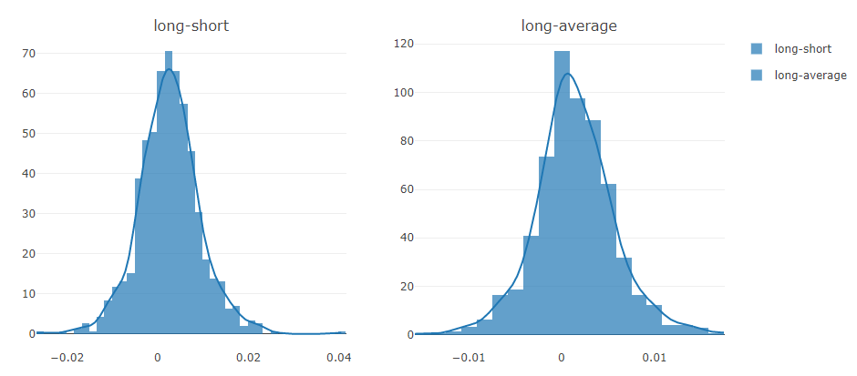
备注

• long-short/long-average

  每个交易日的 long-short/long-average 收益分布

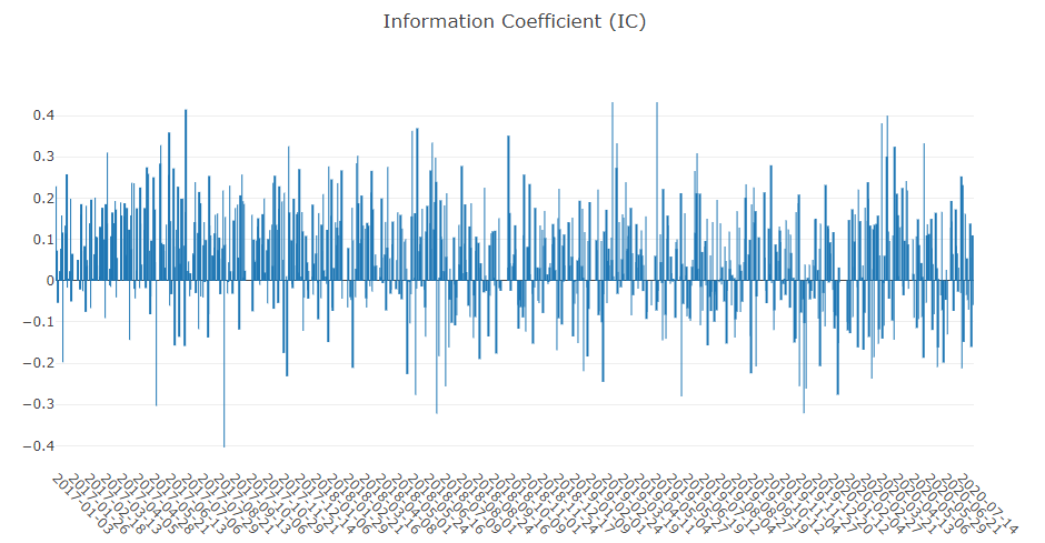
备注

• 信息系数（IC）

  • 投资组合中股票的`labels`与`prediction scores`之间的皮尔逊相关系数序列。

  • 图形报告可用于评估`prediction scores`。

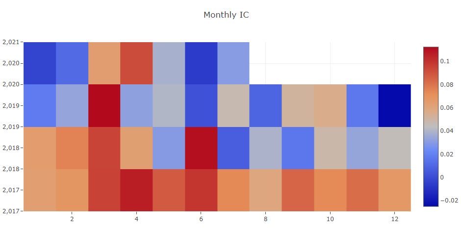
备注

• 月度IC

  月度平均信息系数（IC）

备注

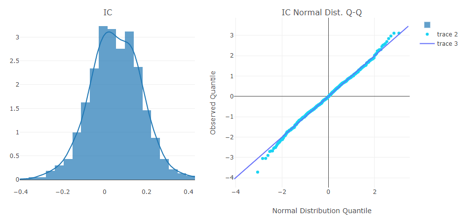
• IC

  每个交易日的信息系数（IC）分布。

• IC 正态分布 Q-Q 图

  Q-Q 图用于展示每个交易日信息系数（IC）的正态分布。

备注

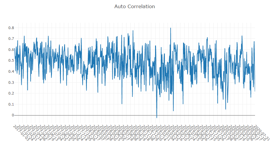
• 自相关

  • 投资组合中股票最新`prediction scores`与`lag`天前`prediction scores`之间的皮尔逊相关系数序列。

  • 图形报告可用于估算换手率。